The simulator of circular dichroism spectra of proteins:
How was it made?

Starting data

Canonical spectra of alpha helix, beta strand, turn and random coil.

The initial datum was the image file ss_960531_AFrame_62 from PPS'96 (Principles of Protein Structure Using the Internet) (availaible in several sites, like:

• The Principles of Protein Structure '97
  http://www.med.unibs.it/~marchesi/pps97/course/section8/ss-960531_21.html#HEADING25
  • http://www.med.unibs.it/~marchesi/pps97/course/section8/ss_960531_AFrame_62.gif
• The Principles of Protein Structure '97
  http://www.cryst.bbk.ac.uk/pps97/course/section8/ss-960531_21.html#HEADING25
  • http://www.cryst.bbk.ac.uk/pps97/course/section8/ss_960531_AFrame_62.gif

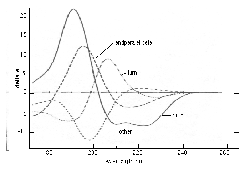
Figure 23. Circular dichroism spectra of "pure" secondary structures. Redrawn from Brahms & Brahms, 1980.

Brahms, S. & Brahms, J. (1980) Determination of protein secondary structure in solution by vacuum ultraviolet circular dichroism J. Mol. Biol. 138, 149-178.

Semi-manually digitised using Engauge Digitizer (from SourceForge, http://digitizer.sourceforge.net/) [According to the record of versions in SF, it should be v. 2.12]

It produced data (X,Y) files, in comma-delimited format (CSV).

They were smoothed in SigmaPlot using Transforms > Smooth 2D data >

• Smoother = Negative exponential
• Sampling proportion = 0.2
• Polynomial degree = 4

I tried to fit data to 3 gaussian curves; alpha and beta were fitting quite well, but I did not use that.

With the interpolate function, data sets were generated with X values in common and regularly spaced:

• interv=data(170,255,1)
• col(15)=interv
• col(N)=interpolate(col(A),col(B),interv)
• donde N=16 a 19, A=1 a 7, B=2 a 8

They overlapped very well with the example spectra,

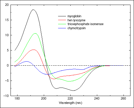
Figure 22. Circular dichroism spectra of triosephosphate isomerase (H:0.52, S:0.14, T:0.11, O:0.23), hen egg lysozyme (H:0.36, S:0.09, T:0.32, O:0.23), myoglobin (H:0.78, S:0.0, T:0.12, O:0.10), and chymotrypsin (H:0.10, S:0.34, T:0.20, O:0.36).

And with these I could create a function that generates combined spectra.

Implementation in the web page:

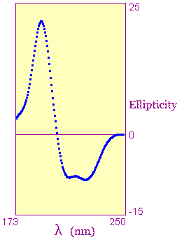An initial version was based on the graphical method by Jeffrey Clymer (rather rewritten):

• http://members.nuvox.net/~on.jwclymer/graphs/plot.html ==> Please go to: http://home.cincyarts.org
• Graphing in JavaScript. Plots functions of your choosing.
  http://home.fuse.net/clymer/graphs/plot.html
  [ jwclymer@one.net Debut: December 26, 2003. Revision No. 3. Wednesday, December 29, 2004 ]

This worked well, but produced dotted lines.

Therefore, a different method was adopted: using the JavaScript graphic library by Walter Zorn to achieve the plot in the figure:

• http://www.walterzorn.com/jsgraphics/jsgraphics_e.htm

Data used to build the plots are:

• the digitised canonical (lists of X,Y values) were exported to CSV format and converted into JavaScript data matrices, which are used in the page to calculate a series of y values (pixels on the screen) for each X (pixels on the screen);
• to generate any combination of secondary structures, a linear combination is made with the canonical spectra, weighted with the fraction of each type of secondary structure;
• for the example proteins, data were taken from the footnote of figure 22 in PPS (see above);
• all this, using JavaScript.